Sparse attention is easy to talk about and hard to ship. The question that actually matters isn’t “is attention sparse?” — it’s which structure you can exploit cheaply enough that the win survives contact with a GPU kernel.
Two papers attack this from opposite directions:
- LServe starts from the serving system and asks: what sparse mechanisms can I plug in at prefill and at decode that give real throughput?
- SampleAttention starts from the attention map and asks: what sparse patterns actually show up in real models, and how do I select them without running dense attention first?
Read together they fit: SampleAttention gives you the map of where sparsity lives; LServe gives you the system that exploits it.
TL;DR
- LServe: different sparse mechanisms for different bottlenecks. Prefill skips KV blocks. Decode prunes KV pages.
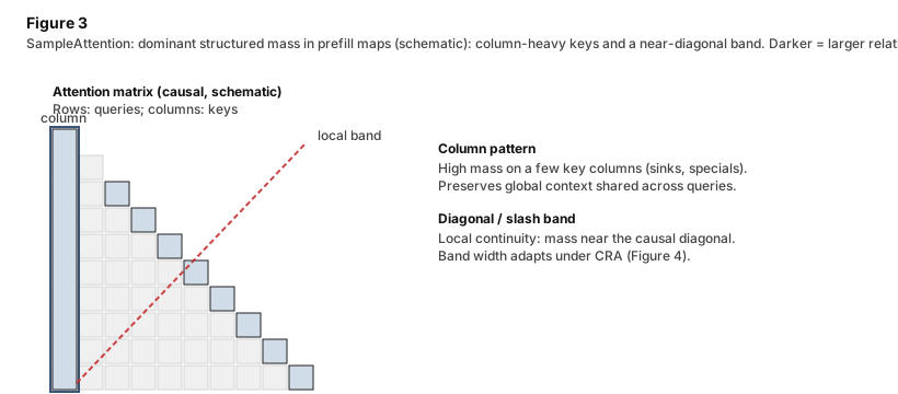
- SampleAttention: two patterns explain most of the important attention mass during prefill. Columns = global anchors. Slashes = local continuity.
- CRA: a runtime accuracy guardrail. Measures how much attention mass your sparse mask actually keeps. No offline profiling required.
Why Fine-Grained Sparsity Doesn’t Work
Both papers start by rejecting the same naive idea: drop arbitrary individual scores below some threshold, get a faster kernel.
The problem is GPU execution. Attention kernels iterate sequentially over KV blocks. Skipping a few scalar operations inside a block doesn’t save iterations — the block still has to be loaded. Unstructured sparsity looks good on FLOPs and bad on actual wall-clock time.
Both papers land on the same fix: exploit structure that aligns with how GPUs already process attention.
LServe — Prefill Phase
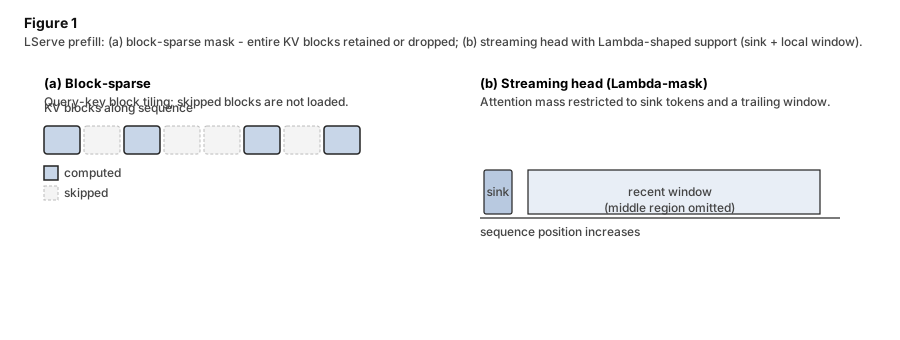
The prefill bottleneck is sequential KV iterations. You have a long prompt, many query tokens, and each needs to walk the KV history. The speedup has to come from reducing how many KV blocks each query touches, not from finer-grained skipping within blocks.
LServe’s approach: block-sparse attention where each block is either fully kept or fully skipped. No partial blocks. This is an important design call — it’s exactly the granularity that maps to the kernel’s iteration structure.
On top of that, LServe converts roughly half the heads into streaming heads with a Λ-mask. A streaming head only keeps recent tokens plus a small set of sink tokens. It never touches the bulk of the KV history. These heads are almost free — they skip the expensive middle of the attention computation entirely.
So prefill is doing two things simultaneously:
- Block-level skipping on the heads that still run full attention.
- Lambda-mask on half the heads so they don’t run full attention at all.
Both still go through unified kernels, not separate code paths.
LServe — Decode Phase
Decode is a different problem. Each step is one query token attending to the full KV cache. There’s no quadratic cost, but there’s a serious bandwidth cost: loading the KV cache from HBM every single step. At 128K context, that’s a lot of data movement per generated token.
LServe’s claim is that for any given query token, you don’t need the full KV cache. Only a small number of pages are actually relevant, and that count stays roughly constant even as context grows. So instead of loading everything, you select the important pages.
The mechanism: a hierarchical page selector scores all pages cheaply using a summary vector per page, picks the top-k, then does fine-grained attention only within those. Selection results are reused across a small window of decode steps to avoid paying the selection cost on every single token.
Combined with INT4 KV quantization, the gains stack: sparsity cuts the number of pages you touch; quantization cuts the byte cost of each page you do touch.
Prefill and decode are genuinely different optimization problems. LServe treats them that way.

SampleAttention — What Sparse Patterns Are Real
SampleAttention focuses on prefill, specifically the TTFT (time to first token) problem at long context. Its core empirical point: attention patterns vary across heads, layers, and prompts, but two structures dominate in almost every setting.
Column Pattern
Certain key positions attract high attention from many different query positions — a whole column of the attention matrix lights up. These are the attention sinks: globally important tokens (separators, special tokens, early context) that many queries want to keep regardless of what they’re looking for.
If you’re going to keep any sparse structure, keep the hot columns. That’s where the long-range global information lives.
Slash Pattern
Query tokens tend to attend to keys near them in the sequence — diagonal or near-diagonal structure. This is local context: the token next to yours matters more than the token 10K positions back. In the attention matrix, that shows up as a slash-shaped band tracking the diagonal.
Columns + slashes together cover a surprisingly large fraction of the attention mass in real models. The paper doesn’t need a long catalog of special cases — just these two.
CRA — The Accuracy Proxy
Most sparse attention papers tune for a fixed sparsity ratio. SampleAttention uses a different control knob: Cumulative Residual Attention (CRA).
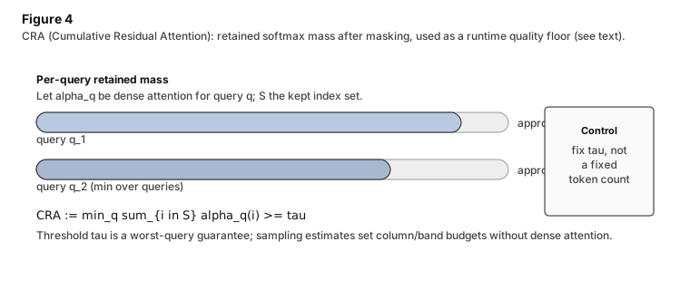
CRA measures, for each query, how much of the original attention probability mass remains after applying the sparse mask. Then it takes the minimum across all queries.
That last part matters. It’s not asking whether the average query kept enough. It’s asking whether the worst-case query kept enough. One badly damaged query can degrade a generation even if 99% of queries are fine.
The practical benefit: CRA lets you set a quality floor instead of a sparsity budget. You say “no query should lose more than 10% of its attention mass” rather than “always keep 20% of tokens.” On hard prompts where attention is concentrated, the mask expands. On easy prompts, it shrinks. You get adaptivity for free.
How it’s computed without dense attention: SampleAttention samples a few query blocks spread across the sequence. From those sampled queries it accumulates approximate column and slash scores cheaply. It then picks the minimum column/slash budget that hits the CRA threshold, and merges those into the final mask. No offline profiling needed; it adapts per-head, per-layer, per-prompt at runtime.
How They Fit Together
SampleAttention answers the structure question: here are the two patterns that matter, here’s how to identify them cheaply, here’s the accuracy signal that tells you if your mask is good enough.
LServe answers the systems question: now that structured sparsity is real, here’s how you build a serving stack around it — unified kernels that handle both sparse and streaming heads, a KV page-selection mechanism for decode, and KV quantization to amplify the bandwidth gains.
The pairing matters because most sparse attention work stops at prefill TTFT. But production serving can’t stop there. Long outputs shift the bottleneck to decode — and decode needs a completely different sparse mechanism than prefill.
Why It Matters in Production
If you’re building long-context inference infrastructure, the real lesson is that the bottleneck moves over the lifetime of a request.
- At prefill: you’re walking a long KV history over many query tokens. Sparsity needs to cut KV block iterations.
- At decode: you’re repeatedly touching a huge KV cache for one token at a time. Sparsity needs to cut page reads.
Treating both with the same mechanism leaves gains on the table.
Three Takeaways
- Prefill and decode need different sparse mechanisms. They have different bottlenecks; don’t optimize them the same way.
- The useful sparse patterns are column and slash. Column = global anchors. Slash = local continuity. Together they cover most of the mass.
- Use CRA as your accuracy guardrail, not a fixed sparsity budget. It’s adaptive, it’s a worst-case bound, and it runs at inference time.
References
- LServe: Efficient Long-sequence LLM Serving with Unified Sparse Attention: arXiv:2502.14866
- SampleAttention: Near-Lossless Acceleration of Long Context LLM Inference with Adaptive Structured Sparse Attention: arXiv:2406.15486
Related: How KV-Cache Paging Works in vLLM — and Why It Matters for Production